The LEFT, RIGHT guide
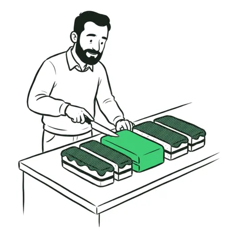
=LEFT(A2, 3) takes the first 3 characters of A2 and =RIGHT(A2, 4) the last 4. For codes with a fixed shape, like CHR-0458, that's all you need to split them.
Syntax
=LEFT(text, [num_chars])
=RIGHT(text, [num_chars])
LEFT counts from the start, RIGHT from the end. Leave num_chars out and you get one character. Ask for more characters than the text has and you get all of it.
Count every character
In CHR-0458 the category is C, H, R: 3 characters. Take 4 and you get "CHR-" with the hyphen. Spaces and punctuation count like letters. When the codes all have the same shape, count once on one code and the same number works for every row.
The result is text
LEFT and RIGHT always give text, even when they cut out digits. For a code that's what you want: "0458" keeps its zero. For a number you mean to add up, it isn't: SUM skips text, and a lookup for the number 458 won't find the text "458". Wrap it in VALUE( ) when you need a number, and leave it alone when it's a code.
When the parts aren't the same length
LEFT and RIGHT with a fixed count only work when every row has the same shape. For names and other text where the length changes, let FIND say where to cut: split first and last names. To take characters from the middle, use MID.
Common mistakes
- Leaving out the count.
=LEFT(A2)gives one letter. - Counting the hyphen. 4 for a 3-letter code brings the hyphen along.
- Turning a code into a number. VALUE or *1 drops the leading zeros.
FAQ
- How do I get the first characters of a cell in Excel?
- Use LEFT: =LEFT(A2,3) returns the first 3 characters of A2.
- How do I get the last 4 characters in Excel?
- Use RIGHT: =RIGHT(A2,4) returns the last 4 characters of A2.
- Why does LEFT return text instead of a number?
- LEFT, RIGHT and MID always return text. Wrap the result in VALUE to turn it into a number, or keep it as text for codes with leading zeros.
- What happens if I leave out num_chars?
- LEFT and RIGHT return one character.